Aki Shiroshita (Epidemiology PhD student, akihiro.shiroshita@vanderbilt.edu) developed a tailored version of DeGAUSS specifically for the EV project.
About Original DeGAUSS
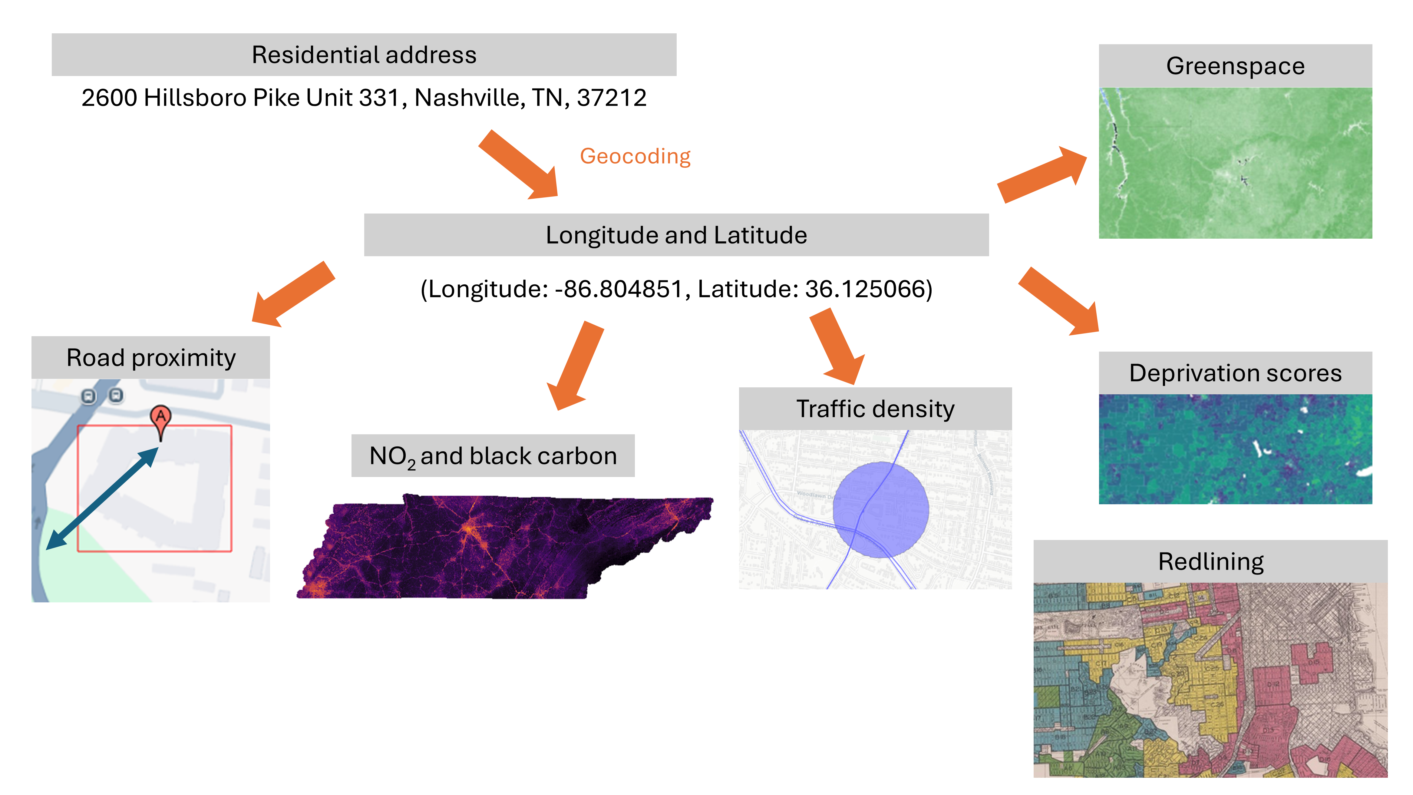
DeGAUSS is designed to derive environmental variables while preserving the privacy of protected health information (PHI). It uses Docker images to process address data, Users upload a CSV file containing address information and receive an output file with various environmental variables.

Limitations of Original DeGAUSS
Original DeGAUSS may not be so flexible.
Not optimized for very large datasets.
Requires input and output files to be stored in the same folder.
Does not support creation of custom variables.
Improvements in the Modified DeGAUSS
Avoid reliance on Docker, using Podman only for part of the process. (VUMC moved from Docker to Podman in October 2025)
Utilize C and C++ in the backend wherever possible.
Enable parallel processing with multiple cores. (Windows OS and Podman setups don’t support FIFOs used by internally in the original DeGAUSS for parallel geocoding)
Restrict environmental data to Tennessee only, not the entire U.S.
Modified DeGAUSS provides clean, processed output files with all PHI removed.
What can we get through Modified DeGAUSS?
| Category | Variable name | Data source | Description |
|---|---|---|---|
| Parsing and normalizing | address |
libpostal | cleaned address |
| Geocoding | lon |
TIGER/Line Street Range Address | longitude and latitude |
lat |
TIGER/Line Street Range Address | longitude and latitude | |
| Road proximity | dist_to_1100 |
U.S. Census Bureau | distance (meters) to the nearest S1100 road |
dist_to_1200 |
U.S. Census Bureau | distance (meters) to the nearest S1200 road | |
length_1100 |
U.S. Census Bureau | length (meters) of S1100 roads within a 500 m buffer | |
length_1200 |
U.S. Census Bureau | length (meters) of S1200 roads within a 500 m buffer | |
| Traffic density | length_moving |
U.S. Department of Transportation Federal Highway Administration | total length of interstates, expressways, and freeways (meters) |
length_stop_go |
U.S. Department of Transportation Federal Highway Administration | total length of arterial roads (meters) | |
vehicle_meters_moving |
U.S. Department of Transportation Federal Highway Administration | average daily number of vehicles multiplied by the length of interstates, expressways, and freeways (vehicle-meters) | |
vehicle_meters_stop_go |
U.S. Department of Transportation Federal Highway Administration | average daily number of vehicles multiplied by the length of arterial roads (vehicle-meters) | |
truck_meters_moving |
U.S. Department of Transportation Federal Highway Administration | average daily number of trucks multiplied by the length of interstates, expressways, and freeways (truck-meters) | |
truck_meters_stop_go |
U.S. Department of Transportation Federal Highway Administration | average daily number of trucks multiplied by the length of arterial roads (truck-meters) | |
| New road proximity and traffic density | dist_near |
U.S. Department of Transportation Federal Highway Administration | distance (meters) to the nearest interstates, expressways, or freeways |
aadt_near |
U.S. Department of Transportation Federal Highway Administration | average daily number of vehicles of the nearest interstates, expressways, or freeways | |
| Redlining categories | redlining |
Mapping Inequality | Historic HOLC classifications (A, B, C, and D) |
| Greenspace | evi_500 |
LP DAAC MOD13Q1 | average enhanced vegetation index within a 500 meter buffer radius |
evi_1500 |
LP DAAC MOD13Q1 | average enhanced vegetation index within a 1500 meter buffer radius | |
evi_2500 |
LP DAAC MOD13Q1 | average enhanced vegetation index within a 2500 meter buffer radius | |
| Deprivation score | fraction_assisted_incom |
2015 American Community Survey | fraction of households receiving public assistance income or food stamps or SNAP in the past 12 months |
fraction_high_school_edu |
2015 American Community Survey | fraction of population 25 and older with educational attainment of at least high school graduation (includes GED equivalency) | |
median_income |
2015 American Community Survey | median household income in the past 12 months in 2015 inflation-adjusted dollars | |
fraction_no_health_ins |
2015 American Community Survey | fraction of population with no health insurance coverage | |
fraction_poverty |
2015 American Community Survey | fraction of population with income in past 12 months below poverty level | |
fraction_vacant_housing |
2015 American Community Survey | fraction of houses that are vacant | |
dep_index |
2015 American Community Survey | composite measure of the 6 variables above | |
| Air pollutants | average_no2_infancy |
Original Schwartz model | Average monthly NO₂ levels during the exposure period |
average_bc_infancy |
Provided by Kai Zhang | Average monthly black carbon levels during the exposure period |
In addition, you can obtain the following information if needed:
Indicator of whether each child experienced relocation and changes in environmental exposures (e.g., moving closer to or farther from major roads).
Number of children per census block (blocks with fewer than 11 children are masked as “<11”).
A wide range of deprivation scores: ADI, SVI, COI, EJI, CRE, DCI, NDI NSES, SDI, and EQI, etc.
Brief description of what Modified DeGAUSS is doing.
modified_degauss_run_xxx.R
This is the main script (index file) that specifies the folder structure and file paths for input and output data. All subsequent scripts are called or sourced from here.
R/initial_set_up.R
This script ensures that Podman is properly configured and running. It also loads all required R packages and custom functions used.
R/xxx_cohort_preparation_simple.R
This script prepares the child cohort data before address standardization and geocoding.
R/xxx_cohort_preparation_simple.R keeps only address
records overlapping with the exposure period, such as infancy (e.g.,
from birth to 1 year).
R/parsing.R
This script parses and normalizes raw addresses using
libpostal to improve match rates in geocoding.
libpostal is a machine learning–based address parser
trained on OpenStreetMap data.
The environment for libpostal is created using Podman, based on ghcr.io/degauss-org/postal:0.1.4.
Each raw address should end with a 5-digit ZIP code, as the geocoding algorithm uses it as the initial search key.
R/geocoding_xxx.R
This is the most time-consuming part of the pipeline. It performs
address geocoding using the Ruby gem Geocoder-US-2.0.4.
The algorithm applies fuzzy matching, and low-confidence results are removed. The Ruby and SQL geocoding environment is built using degauss/geocoder:3.0.
The data source of address is TIGER/Line Address Range files (2021) from the U.S. Census Bureau.
Post-geocoding cleanup
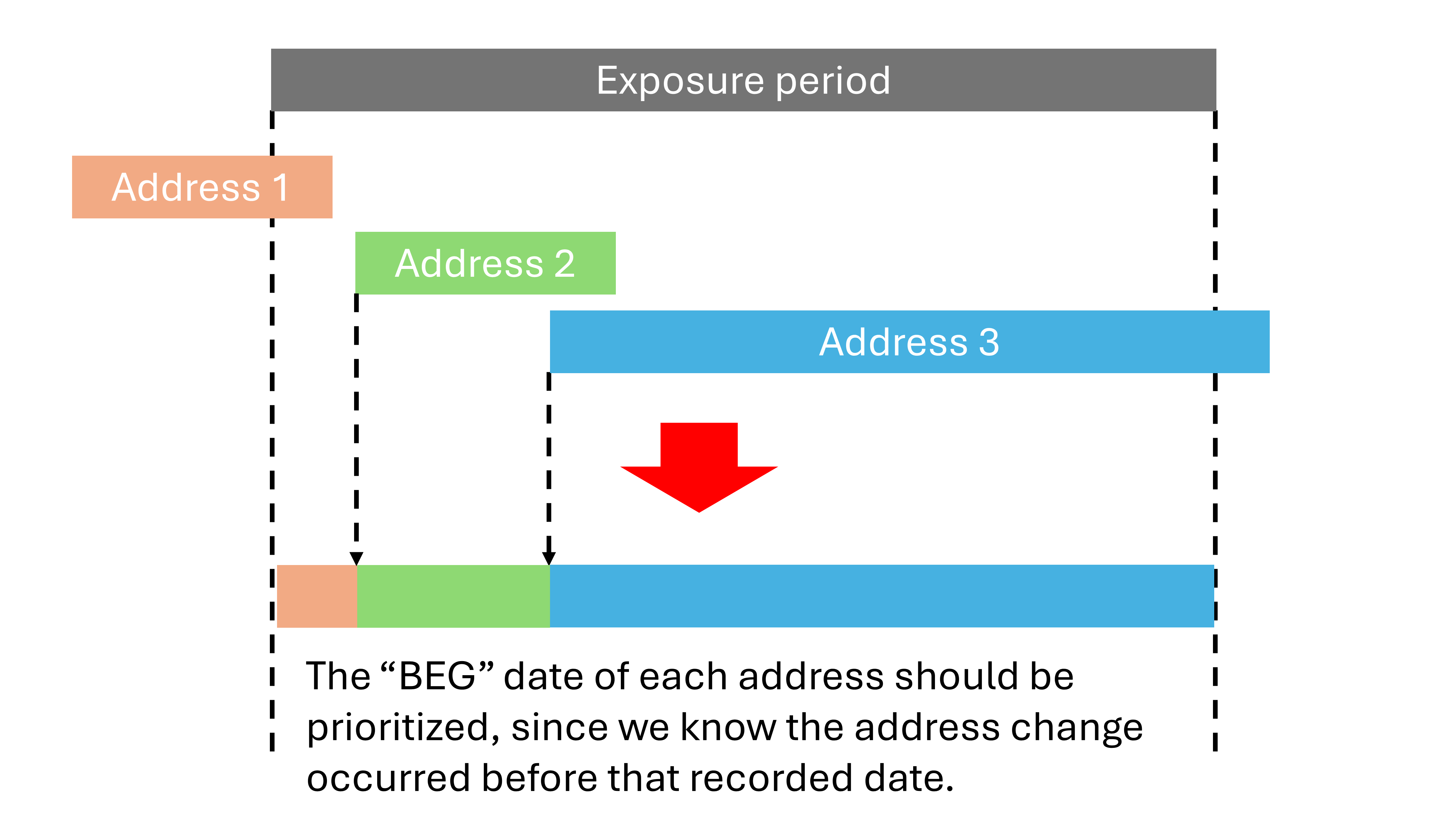
The script then adjusts address timelines to match each child’s exposure period. It creates a single continuous time span, with a total of about 365 days for each child.
- Trimming timeline edges:
The start date of the first address is trimmed so it doesn’t precede the child’s date of birth.
The end date of the last address is trimmed so it doesn’t extend beyond the first birthday.
- Resolving gaps and overlaps:
If a gap exists between consecutive address periods, the end date of the earlier record is set to one day before the next record starts.
If an overlap exists, the end date of the earlier record is adjusted similarly.
R/census.R
This script appends census and redlining variables to each address.
Adds FIPS codes (census tract and block group IDs) for both 2010 and 2020: TIGER boundary files (restricted to Tennessee)
Adds Home Owners’ Loan Corporation (HOLC) redlining grades (A, B, C, D): the University of Richmond
R/road.R
This script calculates the shortest distance to the nearest primary and secondary roads (separately).
Road data are from TIGER 2011, accessed via the R tigris package. The data source is U.S. Census Bureau TIGER/Line Files.
I chose the 2011 data because it is the earliest year for which primary and secondary road shapefiles are available through R tigris package.
R/green.R
This script calculates the average Enhanced Vegetation Index (EVI) around each residential address, which serves as a measure of surrounding greenness.
EVI data are derived from LP DAAC MOD13Q1, a product of NASA’s Land Processes Distributed Active Archive Center (LP DAAC). A cloud-free composite EVI raster at 250 × 250 m resolution was created by assembling individual remote-sensing images collected between June 10 and June 25, 2018, by Professor Cole Brokamp.
R/dep_index.R
This script computes census tract-level material deprivation indices created by Professor Cole Brokamp. The following census tract-level variables were derived from the 2015 American Community Survey:
Fraction of households with income below poverty level within the past 12 months
Median household income in the past 12 months in 2023 inflation-adjusted dollars
Fraction of population 25 and older with educational attainment of at least high school graduation (includes GED equivalency)
Fraction of population with health insurance
Fraction of households receiving public assistance income or food stamps/SNAP in the past 12 months
Fraction of houses that are vacant
Deprivation index: rescaling and normalizing forces the index to range from 0 to 1, with a higher index being more deprived.
For a more comprehensive set of indices, use
dep_index_britt.R, which generates a separate dataset
containing: ADI, SVI, COI, EJI, CRE, DCI, NDI, NSES, SDI, and EQI.
R/aadt.R
This script calculates Average annual daily traffic within a 500-meter buffer radius of each residential address × road length for interstates, expressways, and freeways.
Traffic and road data were obtained from the U.S. Department of Transportation, Federal Highway Administration, using the Highway Performance Monitoring System (HPMS) dataset for 2014, the earliest year available for both vehicle and truck traffic volumes.
It calculates the following metrics:
Total length of interstates, expressways, and freeways (meters)
Total length of arterial roads (meters)
Average daily vehicles × length of moving roads
Average daily vehicles × length of stop-and-go roads
Average daily trucks × length of moving roads
Average daily trucks × length of stop-and-go roads
R/road_and_aadt.R
Because road proximity (from TIGER) and traffic density (from HPMS) are from different data sources, this script integrates both to define a combined exposure metric. It calculates road proximity and Average Annual Daily Traffic (AADT) for interstates, expressways, and freeways using the HPMS dataset, allowing evaluation of the interaction between proximity to major roads and the traffic volume along those roads.
R/road_density.R
This script calculates the length (meters) of primary, secondary and minor roads (separately) within a 500 m buffer radius of each residential address.
Road data are from TIGER 2011, accessed via the R tigris package. The data source is U.S. Census Bureau TIGER/Line Files.
I chose the 2011 data because it is the earliest year for which primary and secondary road shapefiles are available through R tigris package.
R/no2_monthly_xxx.R
This script estimates average NO₂ exposure during the defined exposure period. NO₂ estimates provided by Professor Joel Schwartz are available for 2000-01 through 2016-12.
First, it identify the 1 km² grid cell in which each residential address is located. Then, it pulls monthly NO₂ values corresponding to the address’s grid cell during the exposure period. Finally, compute the mean NO₂ concentration across all months within the exposure window.
R/bc_monthly_xxx.R
This script estimates average Black carbon (BC) exposure during the defined exposure period. BC estimates provided by Professor Kai Zhang are available for 2000-01 through 2017-12.
First, it identify the 0.01° × 0.01° grid cell in which each residential address is located. Then, it pulls monthly BC values corresponding to the address’s grid cell during the exposure period. Finally, compute the mean BC concentration across all months within the exposure window.
R/tabulation.R
This script calculates the number of children per census block group (blocks with fewer than 11 children are masked as “<11”).
R/final_clean_xxx.R
The final data-cleaning step. It removes all PHI, and retains only necessary environmental and contextual variables.
Specifically, address, latitude, and longitude are removed.